Time is complicated. More specifically, the way we record and measure time in terms of seconds, minutes, hours, days, weeks, months, years, leap years, and so on can get kind of messy, especially compared to units like those on a standard metric system.
But time is an extremely common and important dimension in data analysis, including data visualization. In some kinds of analyses we can get away with some simplifications, like measuring everything in the same unit, like second or days or something like that. But especially in data visualization, we may need to communicate different kinds of cycles, like showing the change across different weeks or months or years.
In order to help manage this, this tutorial has two goals. First, I’ll go through a few of the basics of time formats and talk about how to use the lubridate package to convert some of the more common date/time strings into a proper data format. Second, I’ll show you some of the common ways to format time for the purpose of displaying things in plots, like formatting dates on a plot axis.
Standards
Epoch time
The first concept to know about is epoch time. In short, one of the simplest ways to represent a specific moment in time, at least for computers, is a simple count of how many seconds have passed since a particular starting point, called an epoch.
It turns out that for most systems, there is a standard epoch – sometimes referred to as Unix time – that starts at midnight1 on January 1, 1970, in the UTC time zone.2 So a value of 1 would be one second after midnight on Jan 1, 1970, and so on. In practical terms, this can mean that sometimes if you coerce a datetime value into a numeric value, it will get converted into a large number. For example, midnight of January 1, 2025 is 1,735,689,600 seconds after the beginning of the epoch. So if you think you’re working with a datetime value but you’re seeing values close to a billion, that’s likely an indication that you’re dealing with epoch time, in seconds.
1 Just to be super clear, by “midnight”, I mean the instant that the date changed from Dec 31, 1969 to Jan 1, 1970. That’s the zero value.
2 Another interesting piece of trivia is that “UTC” is an acronym that doesn’t exactly stand for anything, because it represents a compromise. This time zone is the one that corresponds to the UK, and earlier in history it was called “Greenwich Mean Time” (GMT). The UTC label stands for “Coordinated Universal Time” in English, but “Temps Universel Coordonné” in French, and when it was designated as a new universal standard, the organizations responsible wanted the three-letter code to be universal across all languages. So as a compromise, instead of picking CUT or TUC or something based on a specific language, the decision was made to use UTC for all languages.
POSIX
Another important acronym to be aware of is POSIX. This refers to a family of standards across many aspects of computing, not just time standards. But in R, some of the datetime classes have “POSIX” in the name, like “POSIXct” or “POSIXt”. This is also related to epoch time (the POSIXct class essentially still captures the values in epoch time), but if you see your time data represented as these classes, that’s good.
Common date string formats
One of the POSIX standards is a set of common symbols used to represent different kinds of date formats. Think about how many different ways dates can be written in English. For example, the following all refer to the same date:
January 13th, 2025
Jan 13, 2025
13 Jan 2025
01/13/2025
1/13/25
2025-01-13
… and so on. There are full month names, abbreviations, different orders, different separating characters, etc. etc. So part of what POSIX did was to designate a common set of symbols (characters) that represent these different “chunks” of a written date. In R, these are all preceded by a % as well. Here’s a non-exhaustive list of the most common ones:
Date/day format symbols
symbol
represents
%d
day of the month with a leading zero (01, 02, 03 … 31)
%e
day of the month without a leading zero (1, 2, 3 … 31)
3 Just by the way, some systems also represent day of the week as an integer, and depending on the system, locale, or other settings, day 1 might be Sunday or Monday. Sunday is probably the most common default.
Time format symbols
symbol
represents
%H
hour in 24-hour format (00-23)
%I
hour in 12-hour format, with leading zero (01, 02 … 12)
%i
hour in 12-hour format, no leading zero (1, 2 … 12)
%p
AM/PM
%M
minute
%S
second
%Z
time zone name (UTC, etc.)
%z
UTC offset (+/- HHHH)
Locales
String formatting of time also depends on the locale (sometimes also called localization), which is a technical term that is used to distinguish what are either different geographic or linguistic regions. For example, the month names and abbreviations are obviously different in English, Spanish, and Chinese. Bit the format symbols above are still correct. So the precise output is a combination of the format strings used, interpreted according to the locale of the machine producing the output.
Using lubridate to make your life easier
The basic problem
Despite all of the standards discussed above, whenever you come across data that contains times, dates, or datetimes, it’s rarely predictable what exact format it will take. Converting what are typically strings of text into proper datetime objects is a necessary step for analysis, including visualization, but since the string formats can have a wide variety of forms, there can’t be a simple uniform solution.4
4 One example of an “unsolvable” challenge for a simple algorithm would be when you are looking at date ranges that are ambiguous in terms of numerical values for days/months/years. For example, given a string like “09-03-12”, American conventions of month-day-year would indicate September 3, 2012, European conventions of day-month-year would indicate March 9, 2012, but it’s also possible it could be in descending order of year-month-day, indicating March 12, 2009. Knowledge of the source of the data or the intended date range might be needed to disambiguate something like this.
This means that the best solution might me to provide a tool for analysts that they can use to apply their own judgment on the structure of the format, to easily convert from “families” of similar string formats into a proper data format.
The lubridate easy button
For this purpose, the lubridate package is a gift, besides being one of the best-named R packages of all time.5 This package provides a number of capabilities for enhancing how R treats datetime objects, but one of the best is its family of {ymd}_{hms}() functions.
5 In my mind, the cleverness of the lubridate name is second only to the referential genius of the magrittr package.
In short, lubridate has a series of functions whose function names serve essentially as a shorthand for different datetime format string patterns. For example, the ymd_hms() function takes a string that follows the “YearMonthDay_HourMinuteSecond” format, handling all varieties of different abbreviations, leading zeros, separating strings, AM/PM or 24-hour formats, and so on. But even better, there are different versions of these functions that simply differ in the order of the characters in the function name, to indicate different orderings in the format string. Additionally, the underscore is optional, so that you can use either “half” of the sequence to format simple dates or simple times.
See the examples below:
library(lubridate)
Attaching package: 'lubridate'
The following objects are masked from 'package:base':

    date, intersect, setdiff, union
print(ymd_hms("2015-09-22 13:22:45"))
[1] "2015-09-22 13:22:45 UTC"
print(ymd_hms("2015-09-22 1:22:45 PM"))
[1] "2015-09-22 13:22:45 UTC"
print(ymd_hm("2015-09-22 13:22"))
[1] "2015-09-22 13:22:00 UTC"
print(ymd_h("2015-09-22 1PM"))
[1] "2015-09-22 13:00:00 UTC"
print(mdy_hm("Sep 22, 2015 13:22"))
[1] "2015-09-22 13:22:00 UTC"
print(mdy_hm("Sep 22nd, 2015 13:22"))
[1] "2015-09-22 13:22:00 UTC"
print(mdy_h("09/22/15 1PM"))
[1] "2015-09-22 13:00:00 UTC"
print(mdy("09/22/15"))
[1] "2015-09-22"
print(hms("The event took 10 hours, 13 minutes, and 45 seconds"))
[1] "10H 13M 45S"
print(hm("1:13 PM"))
[1] "1H 13M 0S"
The final example shows that the {hms}() functions parse strings into “period component” objects, not strictly “time of day”-type objects. This means they do not manage AM/PM, so if you wanted to compute/plot differences or progressions in the hours of the day, you would need to use a 24-hour format.
But with all of the datetime functions that include some part of a {ymd} component, tey handle a wide variety of string formats without the need to refer to the nitty-gritty of the POSIX standard formatting strings described above.
In short, if your task is to simply take datetime data represented in some kind of string format and convert those strings into proper datetime objects, the {ymd}_{hms}() family of functions make that incredibly easy.
Using format strings and date time scales in ggplot2
However, if you want to visualize your data in ggplot2 and you want to control the formatting of how datetimes are displayed in your plots, you will need to work with format strings.
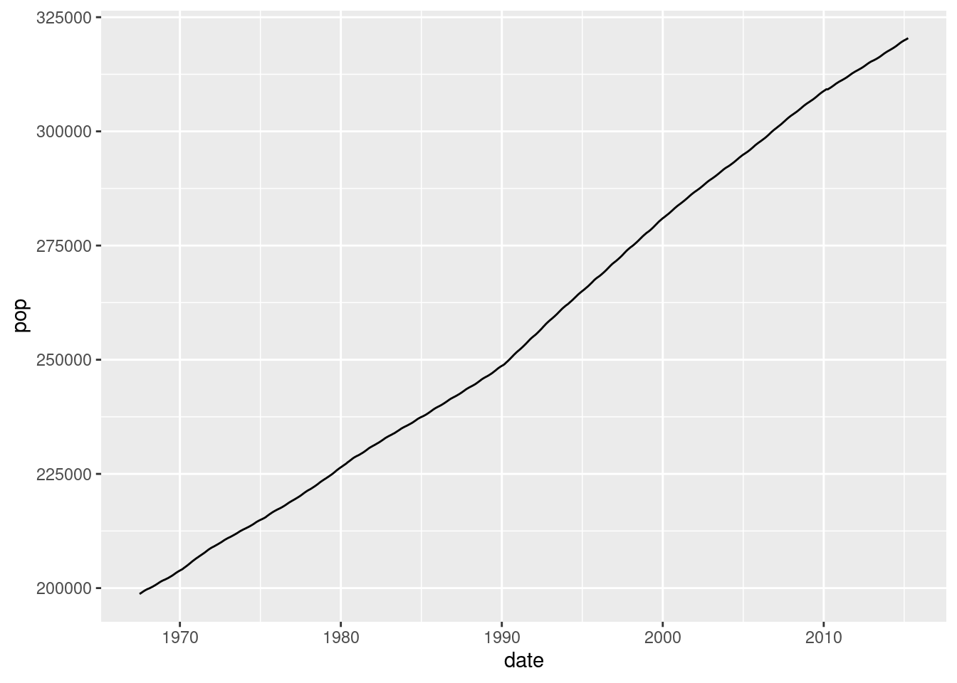
For an example, let’s consider the economics data set that comes pre-loaded in the ggplot2 package. This data set has a few statistics from the US Federal Reserve like population and unemployment figures (both recorded in units of thousands), but our main interest here is that the date column represents dates from July 1967 to April 2014, in YYYY-MM-DD format (all starting on the 1st of the month). These dates are already in a date data format, so our concern here is changing the format they are displayed in, when we visualize the data.
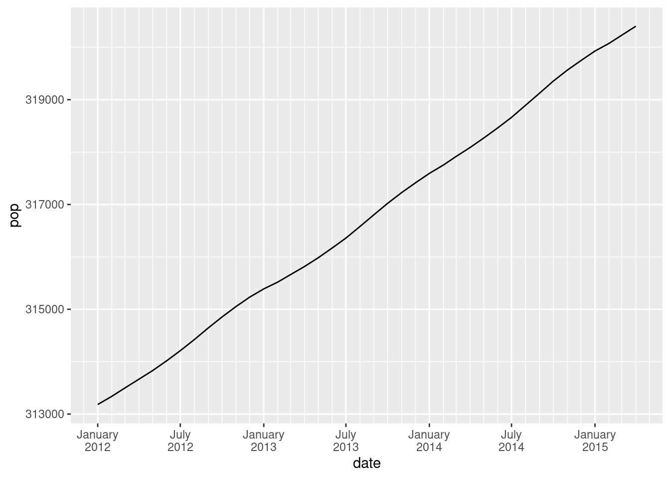
First, let’s examine a simple plot of population over time:
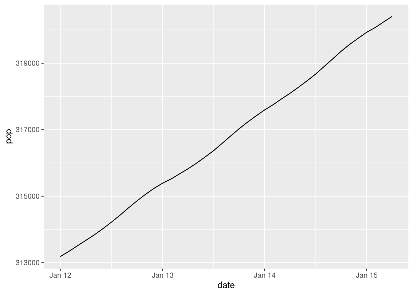
Let’s zoom in a bit on a period where we can examine changes between months. For this, we can subset the data using the filter() function from dplyr, but using the handy lubridate functions discussed above when designating which rows to keep, basically keeping all of the data since the start of 2012.
library(dplyr)
Attaching package: 'dplyr'
The following objects are masked from 'package:stats':

    filter, lag
The following objects are masked from 'package:base':

    intersect, setdiff, setequal, union
economics_recent <-filter(economics, date >ymd("2011-12-31"))ggplot(economics_recent, aes(date, pop)) +geom_line()
This shows our new data, but we are still only displaying years on the x-axis. In order to adjust this axis, we can use the scale_x_date() or scale_x_datetime() functions in ggplot2. Like other scales, these have breaks and labels arguments, but they also have specialized date_breaks and date_labels objects that essentially provide shortcuts to working with dates.
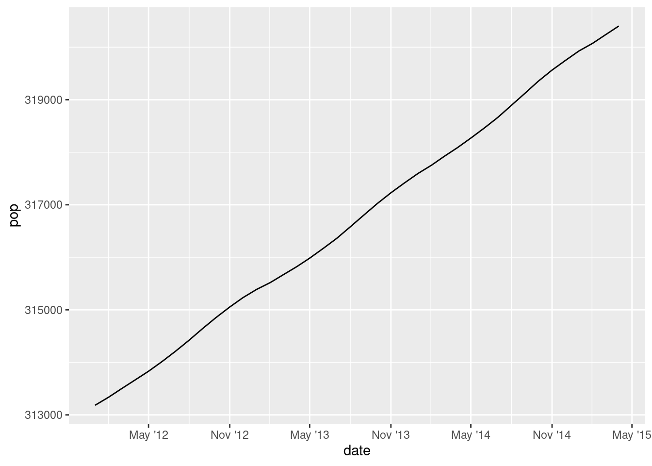
For example, we can use the POSIX standard format strings with the date_labels argument to specify exactly how the dates should be formatted on the axis. Let’s use the abbreviated month and the year.
This is a little better, but it may be a little confusing showing the year as two digits. But remember that other than the format string symbols, we can add to the format strings to include anything else we want. For example, people often show two-digit years with a leading apostrophe, so that 2012 is abbreviated as ’12. So we can just add that apostrophe to our format string if we want.
Now, what if we would like to display a tick mark every six months? Specifying where the tick marks are is normally a job for breaks, but we can also use date_breaks to be able to specify things in terms of time/date units. For example, here’s how to make breaks every six months:
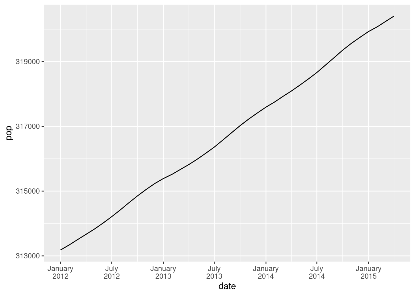
But what if we would like the breaks to fall on specific dates? Here, we might want to force the breaks to occur on January and July instead of May and November. In this case, we can create a sequence of dates using R’s regular seq() function, and we can use lubridate to set the start and end points, and we can specify the by unit in terms of time. Since we are specifying the dates like this with seq(), we just use the normal breaks argument in the scale. In other words, if we want to set breaks “manually”, we pass a sequence of dates to the breaks argument, but if we want to simply specify a length of time between breaks, and have ggplot2 pick the exact break points, we can just use the date_breaks argument to do this more easily.
In addition to setting these breaks, let’s take the opportunity to try another example of a formatting tweak. This time, let’s use the full year and month names, and let’s use the newline character “” to put the month and year on different lines:
In summary, while dates, times, and datetimes can be challenging to work with, the lubridate package makes it very easy to convert strings into proper date/datetime objects, and through the date and datetime scales, ggplot2 gives us a lot of relatively convenient control over the precise formatting of dates in graphical output.
This tutorial is meant to give you a good handle on the essentials, along with examples, but here is some additional documentation for going deeper into these packages and functions:
Pretty version of the documentation of the strptime() and strftime() functions from base R, which includes a more exhaustive listing of format string symbols: https://rdrr.io/r/base/strptime.html